PIV Particle Image Velocimetry: use and benefit

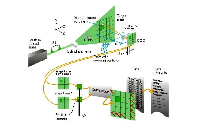
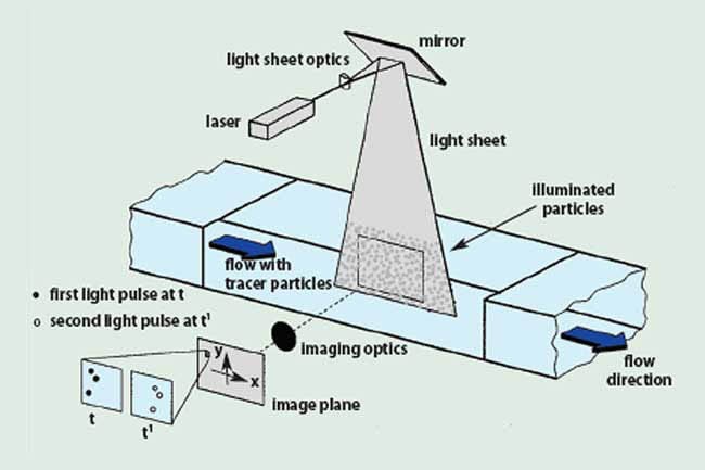
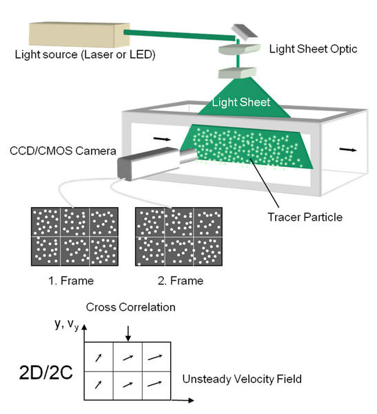
Okay, so today I wanted to mess around with something called “particle image velocimetry,” or PIV for short. It’s basically a way to figure out how fluids are moving by looking at tiny particles in the flow. Sounds cool, right? I thought so too.

First, I needed to get my hands dirty. I realized I will do it with python, So I searched on the internet some useful libraries.

Getting the Tools Ready

I found a few popular libraries, and finally I decided to use OpenPIV.

• OpenPIV:Seemed perfect. Did all the hard work for me.

I installed OpenPiv use `pip install openpiv`.

Setting Up the Experiment (Well, Sort Of)

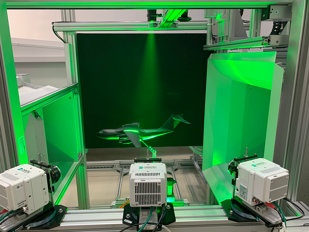
To actually do PIV, you need, like, a flow tank, a laser, a camera, and all that fancy stuff. I didn’t have any of that. So, I did the next best thing: I grabbed some sample images from the OpenPIV GitHub repository. I know, I know, it’s not the real deal, but hey, it’s a start!

Diving into the Code

Here’s where the fun began. I fired up my Jupyter Notebook and started writing some Python code. Honestly, most of it was just following the OpenPIV examples. They made it pretty easy.

Here are my simple code:

from openpiv import tools, process, scaling, validation, filters
import numpy as np
import * as plt
# Load the images (replace with your actual file paths)

frame_a  = *( 'frame_*' )
frame_b  = *( 'frame_*' )
# Define the window size and search area
winsize = 32
searchsize = 64

overlap = 16
# Perform the PIV analysis
u, v, sig2noise = *_search_area_piv( frame_a, frame_b, 
window_size=winsize, overlap=overlap, dt=1, search_area_size=searchsize, 
sig2noise_method='peak2peak' )

# Scale the results (if you know the pixel size and time interval)
# u = u  scaling_factor
# v = v  scaling_factor
# Validate the results (remove bad vectors)
u, v, mask = *_std( u, v, std_threshold=3)

# Replace invalid vectors with an average
u, v = *_outliers( u, v, method='localmean', max_iter=3, kernel_size=3)
# Create a quiver plot to visualize the velocity field
x, y = *_coordinates( image_size=frame_*, window_size=winsize, overlap=overlap )
*(x, y, u, v, scale=50)

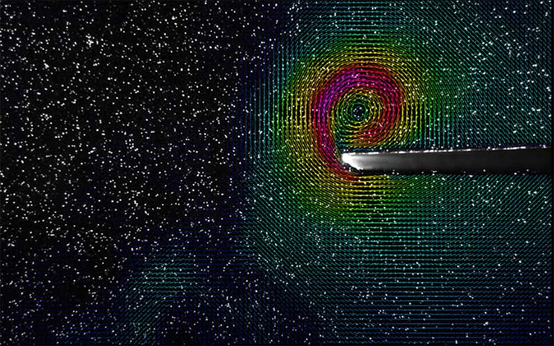
I ran the code, crossed my fingers, and… boom! A vector field appeared! It showed the direction and magnitude of the “flow” between the two images. It wasn’t perfect, there were some wonky vectors here and there, but overall, it looked pretty darn good.

Tweaking and Playing Around

Of course, I couldn’t just leave it at that. I started messing with the parameters: window size, overlap, search area… you name it. I wanted to see how they affected the results. It was like playing with a new toy, except this toy helped me understand fluid dynamics.

I also tried some of the validation and filtering options that OpenPIV provided. These helped clean up the vector field and remove some of the outliers. It’s like magic, I tell ya!

Wrapping Up

So, that was my little adventure with PIV today. I learned a ton, had some fun, and even got a cool-looking vector field out of it. Sure, it wasn’t a groundbreaking scientific experiment, but it was a great way to get my feet wet with this awesome technique. Maybe one day I’ll get my hands on a real flow tank and do some serious PIV analysis. But for now, I’m happy with my sample images and my newfound knowledge.